Reinventing Excel

In Reinventing Discovery Michael Nielsen says that one of the great things about the Internet is the way it can connect problems with problem-solvers. Well, let’s see if that’s true.

I have a problem with Excel, or rather, with a particular spreadsheet that I would like someone to solve elegantly.

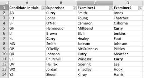
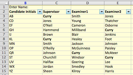
You can download a version of my spreadsheet here. The image below shows the contents. The ‘real life’ spreadsheet will be much bigger but I would like to email it to every person named as a Supervisor, Examiner1 or Examiner2. In principle, each recipient’s name could appear in any of these three columns. I’ve highlighted my own surname to illustrate this.

What I want is a text box at the top of the spreadsheet where each recipient could type their name, an action that would at a stroke reduce the spreadsheet to just those rows that contain their name. I’m guessing this could be done with a macro of some sort. I don’t know. Excel baffles me.

Care to have a try? As an incentive I will send a £10 Amazon voucher to the first person to send me a copy of the spreadsheet that has this function. I promise. You can find me at s dot curry at imperial dot ac dot uk.

OK Internet — go!

Results time — 16th May, 09:00 

Thanks to all the wonderful people who sent in solutions — what an industrious and inventive lot you are. I got solutions from fifteen different people which I wanted to summarise and share. I’m presenting them more or less in order of receipt (with links to the files), which seemed also to track the level of sophistication. At the end, I’ll announce the winner.

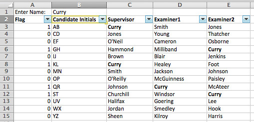
Once of the first entries, from Matthew Russell, hit on a solution that I had implemented crudely myself. The trick is to create an additional column that contains a flag (0/1 or yes/no) to indicate whether the name being searched for occurs in any column:

Having typed in the name you are searching for, you click on the down-arrow attached to the flag column and use the filter function that appears to filter (on ‘1’ in this instance) and so reduce the display to only rows containing that name. Job done. Several others — Dorothy Bishop, Thomas Phillips, Steve Black and Pierre Clavel — came up with similar solutions.

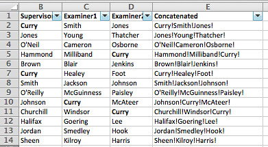
Alan Henness produced a variant on this approach which involves generating a concatenated list of the contents of the columns being searched in a separate column which can then be filtered in the same way as above to find the name you are looking for:

In this case you click on the down-arrow attached to the Concatenated column and filter on the name you are looking for. Peter Binfield also produced a solution like this. It works well but probably would be rather tricky to implement if you had a large number of columns to search.

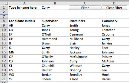
These solutions require the user to invoke the filter command but I was really looking for a simpler solution (not trusting to the Excel capabilities of myself or my users). Siobhan Clibbens came up with a nice button-driven implementation that relies on macros. Here, you type in the name you are searching for and click on the easy-to-spot ‘Filter’ button to show only those rows with the search string. Clicking the ‘Clear Filter’ button resets the spreadsheet to its original form.

Others sent variants of this button approach including Stephen Royle, Kevin Marshall, and @BenMMiles house mate (still nameless!) but to my eye Siobhan’s had the neatest user interface.

Stuart Cantrill sent a slightly modified version of this approach which, rather than relying on buttons, presented instructions on keystroke combinations to control the filtering of the spreadsheet.

Matthew Russell produced a second entry (keen!) that streamlines this approach even further. There are no buttons to press, you simply enter the name you are searching for and hit return. The filtering occurs automatically. To reset, you clear the text entry box and hit return again. Nice.

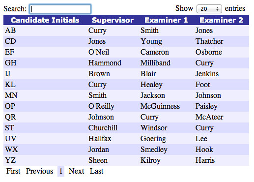
The most radical solution was sent in by Christian Cole who argued strongly on Twitter that Excel is not the tool to be using for this sort of data handling and sent in a web-based solution (zipped file) that relies on HTML and javascript. It works beautifully – the rows of the table (database?) collapse as you type:

I realise I am a lowly Excel neophyte so my commentary on this is almost worthless but I was very impressed by the technical skill on show here. Equally splendid was the willingness of so many people to rise to the challenge. Several commented that they weren’t interested in the £10 prize money, but had simply been driven by the challenge. That’s great news because next time I may not have to offer any reward! 😉

But there has to be a winner and so the prize goes to Siobhan Clibbens for the combination of the particular elegance of her solution and her speed of submission (Update: see below for modifications suggested by Tom Grant that will make it scalable). Honourable mentions to everyone else.

Ultimately, which solution I implement to solve my real-life problem with depend on how easy it is to adapt to the bigger spreadsheets that I have to handle, but I feel I have made some important steps along the learning curve and that a great deal of help is readily available.

Thanks again to everyone who participated. Internet FTW, as I believe people like to say.

Update 18th May, 11:13 — Tom Grant emailed to provide a method for adapting the winning solution to make it work for any length of spreadsheet:

‘Open the VBA editor in Excel (Tools > Macro > Visual Basic Editor) and then select “Module 1” from the Project bar on the right, the code should show as follows:

——————————

Sub Filter() ‘ ‘Filter Macro ‘Advanced filter across columns B, C and D so that only rows where the name in cell B1 appears in one of these columns are shown.

‘ Keyboard Shortcut: Ctrl+f ‘ Range(“C10”).Select Range(“A8:D21”).AdvancedFilter Action:=xlFilterInPlace, CriteriaRange:= _ Range(“A3:D6”), Unique:=False End Sub Sub Clear() ‘ ‘Clear Macro ‘ ‘ Keyboard Shortcut: Ctrl+Shift+C ‘ ActiveSheet.ShowAllData End Sub

——————————If you replace the line

Range(“A8:D21”).AdvancedFilter Action:=xlFilterInPlace, CriteriaRange:= _

with

Range(“A8”, Range(“A8”).End(xlToRight).End(xlDown)).AdvancedFilter Action:=xlFilterInPlace, CriteriaRange:= _

this will make it good to go for all list lengths.’

Thanks Tom!

Update 19th May, 13:45 — Some people just can’t stop themselves. Steve Black has re-worked Matthew Russell’s second solution (mentioned towards the end of the blogpost) to make it work for any size of table. If I have understood correctly, Steve’s solution is an ‘Excel Binary Workbook’ (hence the .xlsb extension on the filename) and relies of some Visual Basic code, which you can access from the menu Tools > Macro > Visual Basic Editor.

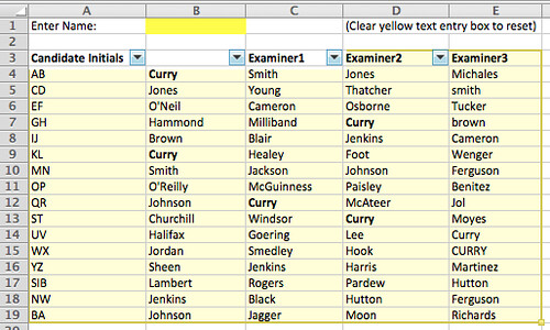
I’ve tweaked it slightly, to add a spacing row at the top and a short instruction on how to reset. Adding the spacing row necessitated a small edit of the code. My changes are in bold below – I set the ActiveSheet.Range (the area highlighted in pale yellow) to start at cell a4 and subtracted 3 from the UsedRange.Rows.Countin the same line to take account of the fact that there are now 3 rows in the spreadsheet before you get to the data that are to be analysed:

Private Sub Worksheet_Change(ByVal Target As Range) If Not Intersect(Target, Target.Worksheet.Range(“b1”)) Is Nothing Then Call HideRows(Target) End Sub

Sub HideRows(TargetName As Range)
Dim cell As Range, rTable As Range

‘set rTable to be active range of table
Set rTable = ActiveSheet.Range(“a4“).Resize(UsedRange.Rows.Count – 3, UsedRange.Columns.Count)

‘unhide all if no name supplied
If ActiveSheet.Range(“b1”).Text = “” Then
rTable.Rows.Hidden = False
Exit Sub
End If

‘hide all
rTable.Rows.Hidden = True

‘only unhide if match found
For Each cell In rTable.Cells
‘test whether cell contains required (ucase ensures capitalisation doesn’t matter); NB also checks student row for simplicity–this might have side effects
If UCase(cell.Value) = UCase(TargetName.Value) Then
cell.EntireRow.Hidden = False
End If

Next

End Sub

Steve recommends cutting and pasting your real-life data into a copy of this spreadsheet to replace the dummy data. To ensure the above version works, you will need to have the data start in cell a4 and have only 3 rows above for your text and headers. Otherwise, you’ll need to edit the code as I have above.

Update 25th May, 13:18 — Steve Black has made a further tweak to his spreadsheet, to allow you to search with strings containing wild cards. Previously it only found exact matches. In the new version a search for *Curry* will return every row that contains Curry (e.g. Curry, Stephen Curry, Beef Curry). The search is not sensitive to case.