
![]() Just before Christmas I was asked to talk to our molecular biologists about multivariate analyses. I was reminded of this on Thursday afternoon, when I saw that I had to talk to them on Friday. “Ah, no problem”, I thought. “I can put something together in the morning. What time is the meeting? 11am? Eek.”
Just before Christmas I was asked to talk to our molecular biologists about multivariate analyses. I was reminded of this on Thursday afternoon, when I saw that I had to talk to them on Friday. “Ah, no problem”, I thought. “I can put something together in the morning. What time is the meeting? 11am? Eek.”
So, I turned up with half an idea about what I was going to talk about, and had the great fortune that the room had a blackboard. And chalk. Several colours of chalk. What fun I had! But I made the mistake of saying I would blog it afterwards, and include some resources for further reading. Well, this is the blog post, and if anyone wants to add more resources, please go ahead in the comments.
I was asked to particularly talk about 2 methods: Principal Component Analysis and Principal Coordinates Analysis. Which, in some ways, was neat because they cover two of the main mathematical approaches to multivariate analyses. I think the main use of these methods is to visualise the data, but more complicated analyses can be done using the same ideas (e.g. MANOVA and factor analysis are based on the PCA approach).
Principal Component Analysis: PCA
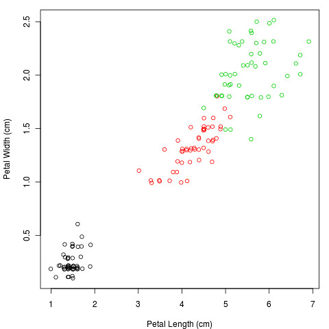
PCA is a statistical yoga warm-up: it’s all about stretching and rotating the data. I’ll illustrate it with part of a famous data set, of the size and shape of iris flowers. The original data has 4 dimensions: sepal and petal length and width. Here are the petal measurements (the different colours are different species):
The purpose of PCA is to represent as much of the variation as possible in the first few axes. To do this we first centre the variables to have a mean of zero:
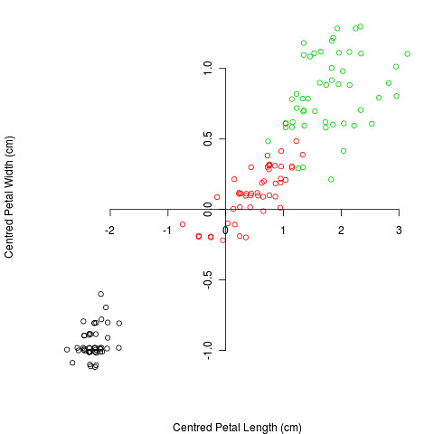
and then rotate the data (or rotate the axes, but I can’t work out how to do that in R):

The rotation is done so that the first axis contains as much variation as possible, the second axis contains as much of the remaining variation etc. Thus if we plot the first two axes, we know that these contain as much of the variation as possible in 2 dimensions. As well as rotating the axes, PCA also re-scales them: the amount of re-scaling depends on the variation along the axis. This can be measured by the Eigenvalue, and it’s common to present the proportion of total variation as the Eigenvalue divided by the sum of the Eigenvalues, e.g. for the data above the first dimension contains 99% of the total variation.
We can also ask how much each variable contributes to each dimension by looking at the loadings, e.g. for the data above we have these:
| PC1 | PC2 | |
|---|---|---|
| Petal Length | 0.92 | -0.39 |
| Petal Width | 0.39 | -0.92 |
We can plot these on a graph: here we have it for the full data, with both sepals and petals:

The arrows show the direction the variables point, so we can see that the petal variables are pretty much the same (i.e. there is a petal size which affects both equally). Sepal width is the only one that’s different, mainly affecting the second PC. It’s almost at 90° from the sepal length, suggesting they have independent effects.
It’s obvious, looking at the data, that one species (I. setosa) is very different, with smaller petals, and differently shaped sepals
Mathematically, PCA is just an eigen analysis: the covariance (or correlation) matrix is decomposed into its Eigenvectors and Eigenvalues. The Eigenvectors are the rotations to the new axes, and the Eigenvalues are the amount of stretching that needs to be done. But you didn’t want to know that, did you?
Principal Coordinate Analysis: PCoA
The second method takes a different approach, one based on distance. For example, we can take a map of towns in New Zealand:

(I’ve rotated the map, to make it easier later)
The geographical distance between the town is Euclidean (well, almost. And near enough that you won’t notice the difference). But we can also measure the distance one would travel by road between the towns. This would give us another measure of distance. Of course this may not be Euclidean in two dimensions, so we can’t simply plot it onto a piece of paper. Distance-based methods are essentially about finding a “good” set of Euclidean distances from distances that are not a priori Euclidean in those dimensions.
The way principal coordinate analysis does this is to start off by projecting the distances into Euclidean space in a larger number of dimensions. This is not difficult; as long as the distances are fairly well behaved then we only need n-1 dimensions for with n data point. PCoA starts by putting the first point at the origin, and the second along the first axis the correct distance from the first point, then adds the third so that the distance to the first 2 is correct: this usually means adding a second axis. This continues until all of the points are added.
But how do we get back down to 2 dimensions? Well, simply do a PCA on these constructed points. This obviously captures the largest amount of variation from the n-1 dimensional space.
So, for the New Zealand data if we do PCoA on the road distances, we get this:

And, not surprisingly, the maps are fairly close to each other, but not exact.
One wrinkle for the sorts of applications we were discussing for bioinformatics (and which is also important in ecology) is the notion of a distance between two data points. In ecology we work with abundances of species, and the distances between the points need to somehow scale the abundances, so that rarer and more common species . So a plethora of diversity indices have been devised, and it’s not clear which one should be used (unless one is in Canberra or New York, I guess). For added fun, some people think they’re all crap.
For me, these methods are mainly useful for visualising the data, so we can actually see how it’s behaving, and they’re not really very good for making formal inferences. But a lot of the multivariate methods for inference have the same ideas at their core, so understanding these is a good starting point.
But it’s still all about avoiding headaches by not having to think in 17 dimensions.
Some resources
Gower, J.C. (2005). Principal Coordinates Analysis Encyclopedia of Biostatistics : 10.1002/0470011815.b2a13070
Bryan F.J. Manly (2004) Multivariate Statistical Methods: A Primer, Third Edition. Chapman & Hall/CRC Press
Jari Oksanen’s course notes (Jari is the maintainer of the vegan package in R)
The Ordination Webpage
Warton, D., Wright, S., & Wang, Y. (2011). Distance-based multivariate analyses confound location and dispersion effects Methods in Ecology and Evolution DOI: 10.1111/j.2041-210X.2011.00127.x
The R code for this post
Hi! Could you update this so the *.jpg images show up in the browser? Thanks!
Oh poo. They weren’t sent with the rest of my back catalogue.
I’ll try to get it fixed
Yes it would be great to have the images view-able!
Thanks!
Any thoughts yet on updating the post with the JPGs included? The post is one of the top ranking Google hits for “PCA vs PCoA”, but without the images it isn’t much help. Many thanks!
Aagh, sorry. I really should get my arse into gear on this…
Bob
Looking for the update with images as it is interesting to know the difference between PCA and PCoA.
Thanks
Would really love to see the images along with your explanations. Thanks!
Thanks!! Your explanation is very comprehensible : )